The basics: bonding descriptors in diamond#
This example demonstrates how pengwann can be used to calculate the Wannier orbital Hamilton population (WOHP) and the Wannier orbital bond index (WOBI) for the C-C bond in diamond. We will also integrate these descriptors to (roughly speaking) measure the bond strength and bond order.
Note
As referenced in the title above, this example is designed to showcase the basics of pengwann as applied to a simple system. This should be enough to get you started, but for more information regarding additional functionality and alternative workflows, please see the other examples and the API reference.
Step 1: Identifying interatomic interactions#
Within pengwann, the interaction between a given pair of atoms i and j is the sum total of all interactions between the Wannier functions associated with atom i and the Wannier functions associated with atom j. In order to compute bonding descriptors for the C-C bond in diamond, we must therefore first figure out which Wannier functions should be assigned to each carbon atom.
from pengwann.geometry import Geometry

geometry = Geometry.from_xyz(seedname='wannier90', path='inputs')

print(geometry)

for site in geometry:
    print(site)
Geometry
========
Cell
----
[[-1.780373 -1.780373  0.      ]
 [-1.780373  0.       -1.780373]
 [ 0.       -1.780373 -1.780373]]

Assignments
-----------
X0 => (8,)
X1 => (9,)
X2 => (8,)
X3 => (9,)
X4 => (9,)
X5 => (8,)
X6 => (8,)
X7 => (9,)
C8 <= (0, 2, 5, 6)
C9 <= (1, 3, 4, 7)

Site(symbol='X', index=0, coords=array([ 0.26424442,  0.57858402, -0.4214136 ]))
Site(symbol='X', index=1, coords=array([0.17141581, 0.48575541, 0.1714149 ]))
Site(symbol='X', index=2, coords=array([-0.42141344,  0.26424353,  0.57858404]))
Site(symbol='X', index=3, coords=array([0.4857563 , 0.1714135 , 0.17141418]))
Site(symbol='X', index=4, coords=array([0.17141464, 0.17141484, 0.48575593]))
Site(symbol='X', index=5, coords=array([-0.42141478, -0.42141459, -0.4214143 ]))
Site(symbol='X', index=6, coords=array([ 0.57858386, -0.42141294,  0.26424387]))
Site(symbol='X', index=7, coords=array([0.17141299, 0.17141598, 0.17141483]))
Site(symbol='C', index=8, coords=array([0.49999989, 0.49999989, 0.49999989]))
Site(symbol='C', index=9, coords=array([0.24999994, 0.24999994, 0.24999994]))
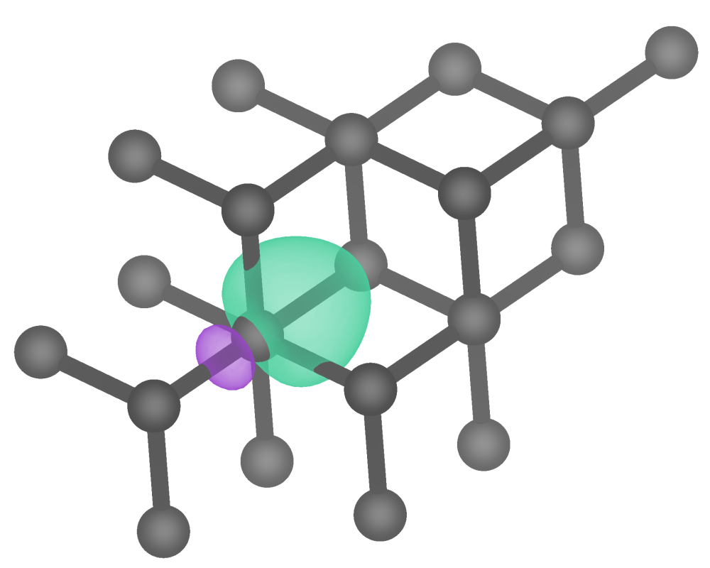
Above, we have initialised a Geometry object using the from_xyz() classmethod, which parses the Wannier90 seedname_centres.xyz and seedname.wout files to extract the coordinates of atoms and Wannier centres as well as the cell vectors. As indicated by the output above, each atom or Wannier centre is represented by an individual Site object and associated with a symbol, index and set of coords (fractional coordinates). For atomic sites, the symbol is just an elemental symbol such as C for carbon, whereas for the sites defined by Wannier centres, the symbol is always X.
In addition to the basic geometric information encoded by Geometry objects, they also assign Wannier centres to atoms based on a closest distance criterion. This is represented in the output above by the Assignments table, which contains indices that associate each Wannier centre with its closest atom. The indices refer to the order of sites in the Geometry object itself, for example, looking at the last site in the structure (a carbon atom at site #9), we read C9 <= (1, 3, 4, 7), meaning that the Wannier centres at sites #1, #3, #4 and #7 have been assigned to this atom. Vice versa, if we look at the first site in the structure (a Wannier centre at site #0), we read X0 => (8,), meaning that this Wannier centre has been assigned to the carbon atom at site #8.
Warning
The seedname_centres.xyz file read by the from_xyz classmethod should always be generated by Wannier90 with translate_home cell = false. If a seedname_centres.xyz file generated with translated_home_cell = true is used, then the Wannier centre assignments will still be accurate, but the interatomic interactions (specifically the Bravais lattice vectors associated with the interacting Wannier functions) identified in subsequent steps may not be accurate.
Now that we have the geometry of the system and its Wannier centres available to us, we can identify interatomic interactions according to a radial distance cutoff:
from pengwann.geometry import identify_interatomic_interactions

# Find all C-C bonds that are < 1.6 Å.
cutoffs = {('C', 'C'): 1.6}

interactions = identify_interatomic_interactions(geometry, cutoffs)

print(interactions)
Atomic interactions
===================
C8 <=> C9
Sure enough, because we are here using the primitive cell of diamond (which contains only 2 carbon atoms), we find just a single C-C interaction between atoms #8 and #9 (with reference to the Geometry generated prior).
The object returned by the identify_interatomic_interactions() function is an AtomicInteractionContainer. As the name suggests, this object is designed to collect multiple AtomicInteraction objects:
for interaction in interactions:
    print(interaction)
Atomic interaction C8 <=> C9
============================
DOS matrix => Not calculated
WOHP => Not calculated
WOBI => Not calculated
IWOHP => Not calculated
IWOBI => Not calculated
Population => Not calculated
Charge => Not calculated


Associated Wannier interactions
-------------------------------
0[0, 0, 1] <=> 1[0, 0, 0]
0[0, 0, 1] <=> 3[0, 0, 0]
0[0, 0, 1] <=> 4[0, 0, 0]
0[0, 0, 1] <=> 7[0, 0, 0]
2[1, 0, 0] <=> 1[0, 0, 0]
2[1, 0, 0] <=> 3[0, 0, 0]
2[1, 0, 0] <=> 4[0, 0, 0]
2[1, 0, 0] <=> 7[0, 0, 0]
5[1, 1, 1] <=> 1[0, 0, 0]
5[1, 1, 1] <=> 3[0, 0, 0]
5[1, 1, 1] <=> 4[0, 0, 0]
5[1, 1, 1] <=> 7[0, 0, 0]
6[0, 1, 0] <=> 1[0, 0, 0]
6[0, 1, 0] <=> 3[0, 0, 0]
6[0, 1, 0] <=> 4[0, 0, 0]
6[0, 1, 0] <=> 7[0, 0, 0]
As we only have one interaction, iterating over interactions just yields one AtomicInteraction object. We can also access the interaction between C8 and C9 via numpy-style indexing:
print(interactions[8, 9])
Atomic interaction C8 <=> C9
============================
DOS matrix => Not calculated
WOHP => Not calculated
WOBI => Not calculated
IWOHP => Not calculated
IWOBI => Not calculated
Population => Not calculated
Charge => Not calculated


Associated Wannier interactions
-------------------------------
0[0, 0, 1] <=> 1[0, 0, 0]
0[0, 0, 1] <=> 3[0, 0, 0]
0[0, 0, 1] <=> 4[0, 0, 0]
0[0, 0, 1] <=> 7[0, 0, 0]
2[1, 0, 0] <=> 1[0, 0, 0]
2[1, 0, 0] <=> 3[0, 0, 0]
2[1, 0, 0] <=> 4[0, 0, 0]
2[1, 0, 0] <=> 7[0, 0, 0]
5[1, 1, 1] <=> 1[0, 0, 0]
5[1, 1, 1] <=> 3[0, 0, 0]
5[1, 1, 1] <=> 4[0, 0, 0]
5[1, 1, 1] <=> 7[0, 0, 0]
6[0, 1, 0] <=> 1[0, 0, 0]
6[0, 1, 0] <=> 3[0, 0, 0]
6[0, 1, 0] <=> 4[0, 0, 0]
6[0, 1, 0] <=> 7[0, 0, 0]
As we can see from the output above, the interaction between C8 and C9 is internally represented by the interactions between their respective Wannier functions. The notation used to refer to each Wannier function can be understood as \(\ket{w_{iR}} =\) i[R_1, R_2, R_3], where i is a band-like index and R_1, R_2 and R_3 are the components of a Bravais lattice vector.
Step 2: Building a DescriptorCalculator#
To actually calculate the WOHP and the WOBI for the C-C bond, we will need to parse a few more Wannier90 input and output files. This can be easily accomplished with the read() function, which parses the Wannier90 seedname.eig, seedname_u.mat and seedname_hr.dat files to yield the k-point mesh, the Kohn-Sham eigenvalues, the unitary matrices that define the Wannier functions and the Wannier Hamiltonian:
from pengwann.io import read

kpoints, eigenvalues, u_matrices, hamiltonian = read(seedname='wannier90',
                                                     path='inputs')
Note
The seedname.eig, seedname_u.mat and seedname_hr.dat files can also be parsed separately by various functions in the io module, the read function is just a convenient wrapper for most use cases.
Optional: Obtain the occupation matrix#
As we would like to calculate the WOBI as well as the WOHP for the C-C bond, we are also in need of the occupation matrix, which is required to compute elements of the Wannier density matrix. Ideally, the occupation matrix should be read directly from the ab initio code, in our case from VASP. Due to the fact that different ab initio codes output the occupation matrix in different formats, pengwann does not provide a generic I/O function for this purpose. We recommend that users look towards larger and more general-use Python packages such as pymatgen or ase for this functionality, and use these to read the occupation matrix from their ab initio calculations.
If for whatever reason, the occupation matrix cannot be read directly from the ab initio code, then the get_occupation_matrix function can be used to reconstruct it from the Kohn-Sham eigenvalues:
from pengwann.occupations import get_occupation_matrix

mu = 10.5 # The Fermi level
nspin = 2 # The number of electrons per fully-occupied state.

occupation_matrix = get_occupation_matrix(eigenvalues, mu, nspin)
Note
By default, the get_occupation_matrix function uses a heaviside function to build the occupation matrix: occupation numbers are 1 below the Fermi level and 0 above it (with a sharp cutoff). In the case of diamond, an insulator, this is perfectly appropriate, but for systems in which thermal smearing has been applied during the ab initio calculation it may be desirable to apply a different occupation function. The get_occupation_matrix function has an optional occupation_function keyword argument that can be used to apply any arbitary occupation function, several of which are available in the occupations module.
The actual calculation of bonding descriptors is accomplished in pengwann via the DescriptorCalculator class.
from pengwann.descriptors import DescriptorCalculator

num_wann = 8
energy_range = (-15, 26)
resolution = 0.1
sigma = 0.2 # Smearing width

dcalc = DescriptorCalculator.from_eigenvalues(eigenvalues,
                                              num_wann,
                                              nspin,
                                              energy_range,
                                              resolution,
                                              sigma,
                                              kpoints,
                                              u_matrices,
                                              h=hamiltonian,
                                              occupation_matrix=occupation_matrix)
The energy_range, resolution and sigma arguments all refer to the manner in which the density of states is to be evaluated: from energy_range[0] up to energy_range[1] in steps of resolution smeared by a Gaussian of width sigma.
Step 3: Integrating and plotting the WOHP and the WOBI#
Having initialised a DescriptorCalculator, actually calculating the WOHP and the WOBI is very straightforward:
interactions = dcalc.assign_descriptors(interactions)
Note that the assign_descriptors() method returns a new AtomicInteractionContainer rather than updating the original in-place - this behaviour is common throughout the pengwann codebase.
print(interactions[8, 9])
Atomic interaction C8 <=> C9
============================
DOS matrix => Calculated
WOHP => Calculated
WOBI => Calculated
IWOHP => Not calculated
IWOBI => Not calculated
Population => Not calculated
Charge => Not calculated


Associated Wannier interactions
-------------------------------
0[0, 0, 1] <=> 1[0, 0, 0]
0[0, 0, 1] <=> 3[0, 0, 0]
0[0, 0, 1] <=> 4[0, 0, 0]
0[0, 0, 1] <=> 7[0, 0, 0]
2[1, 0, 0] <=> 1[0, 0, 0]
2[1, 0, 0] <=> 3[0, 0, 0]
2[1, 0, 0] <=> 4[0, 0, 0]
2[1, 0, 0] <=> 7[0, 0, 0]
5[1, 1, 1] <=> 1[0, 0, 0]
5[1, 1, 1] <=> 3[0, 0, 0]
5[1, 1, 1] <=> 4[0, 0, 0]
5[1, 1, 1] <=> 7[0, 0, 0]
6[0, 1, 0] <=> 1[0, 0, 0]
6[0, 1, 0] <=> 3[0, 0, 0]
6[0, 1, 0] <=> 4[0, 0, 0]
6[0, 1, 0] <=> 7[0, 0, 0]
As seen above, the DOS matrix, the WOHP and the WOBI are now all reported as Calculated (the raw numpy arrays are not displayed because they would take up an impractical amount of screen real estate in most cases).
To evaluate the IWOHP (integrated WOHP) and the IWOBI (integrated WOBI), we call the with_integrals() method:
interactions = interactions.with_integrals(dcalc.energies, mu)

print(interactions[8, 9])
Atomic interaction C8 <=> C9
============================
DOS matrix => Calculated
WOHP => Calculated
WOBI => Calculated
IWOHP => Calculated
IWOBI => Calculated
Population => Calculated
Charge => Not calculated


Associated Wannier interactions
-------------------------------
0[0, 0, 1] <=> 1[0, 0, 0]
0[0, 0, 1] <=> 3[0, 0, 0]
0[0, 0, 1] <=> 4[0, 0, 0]
0[0, 0, 1] <=> 7[0, 0, 0]
2[1, 0, 0] <=> 1[0, 0, 0]
2[1, 0, 0] <=> 3[0, 0, 0]
2[1, 0, 0] <=> 4[0, 0, 0]
2[1, 0, 0] <=> 7[0, 0, 0]
5[1, 1, 1] <=> 1[0, 0, 0]
5[1, 1, 1] <=> 3[0, 0, 0]
5[1, 1, 1] <=> 4[0, 0, 0]
5[1, 1, 1] <=> 7[0, 0, 0]
6[0, 1, 0] <=> 1[0, 0, 0]
6[0, 1, 0] <=> 3[0, 0, 0]
6[0, 1, 0] <=> 4[0, 0, 0]
6[0, 1, 0] <=> 7[0, 0, 0]
Note
The energies property of the DescriptorCalculator class simply returns the discrete energies at which the DOS and all derived descriptors have been evaluated.
We are now in a position to plot the WOHP and the WOBI:
import matplotlib.pyplot as plt

shifted_energies = dcalc.energies - mu

wohp = interactions[8, 9].wohp
iwohp = interactions[8, 9].iwohp

fig, ax = plt.subplots()

ax.plot(shifted_energies, wohp)
ax.fill_between(shifted_energies, wohp, alpha=0.7, where=shifted_energies <= 0)
ax.axvline(x=0, color='black', ls='--', lw=1)

ax.annotate(f'IWOHP = {iwohp:.2f}', (0.25, 0.90), xycoords='axes fraction')

ax.set_xlim(-25, 15)
ax.set_ylim(-1.2, 1.2)

ax.set_xlabel(r'$E - E_{\mathrm{F}}$ / eV')
ax.set_ylabel('WOHP')

plt.show()

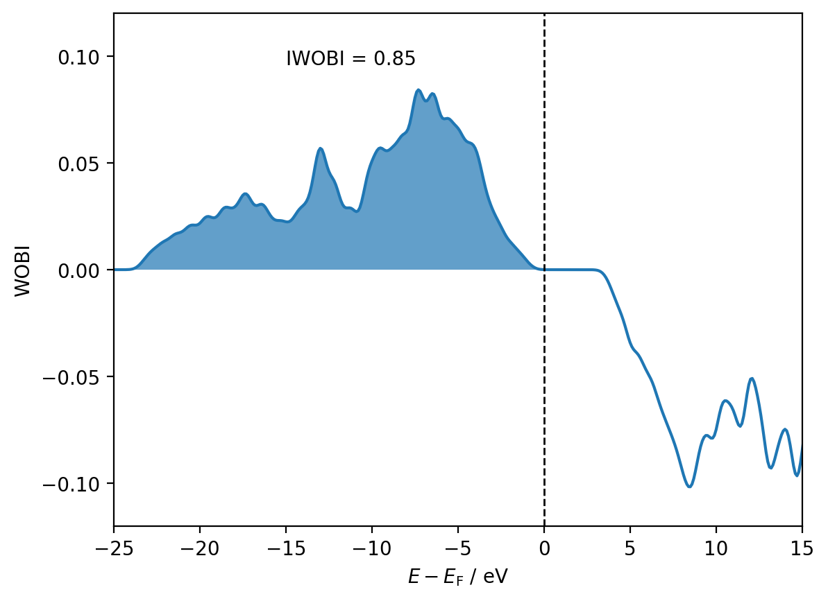
wobi = interactions[8, 9].wobi
iwobi = interactions[8, 9].iwobi

fig, ax = plt.subplots()

ax.plot(shifted_energies, wobi)
ax.fill_between(shifted_energies, wobi, alpha=0.7, where=shifted_energies <= 0)
ax.axvline(x=0, color='black', ls='--', lw=1)

ax.annotate(f'IWOBI = {iwobi:.2f}', (0.25, 0.90), xycoords='axes fraction')

ax.set_xlim(-25, 15)
ax.set_ylim(-0.12, 0.12)

ax.set_xlabel(r'$E - E_{\mathrm{F}}$ / eV')
ax.set_ylabel('WOBI')

plt.show()